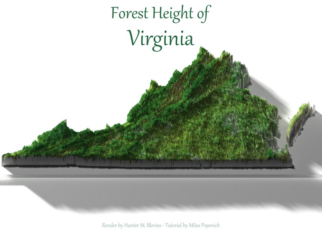
Inspired by the incredible work of Milos Popovic (Blog | Milos Popovic – personal website and blog), I wanted to make the jump to rendered maps. He has a tutorial on using data derived from Google Earth Engine, ggplot2, and rayshader to create stunning forest height maps (youtube.com)
The maps in this project were made in the style of and after following that tutorial. To ensure I’m not repeating steps but genuinely learning, I followed the tutorial video for my first map (not included in this page) and then rewrote the code for each subsequent map.
When writing the code, I prioritized making it easily reproducible when changing areas. This project page will be structured to follow along easily and create your own map. However, if you wish to create your own, I highly encourage you to watch the Milos Popovic tutorial.
To begin with, the required packages are downloaded and loaded using pacman
install.packages("pacman")
pacman::p_load(
  tidyverse,
  geodata,
  sf,
  terra,
  rayshader,
  classInt
)
The Geodata library is used to secure a shapefile for our map
#retrieve country abbreviations from this link - https://www.nationsonline.org/oneworld/country_code_list.htm

get_target_border <- function(){
  main_path <- getwd()
  target_border <- geodata::gadm(
    country="#",
    level = 2,
    path = main_path
  ) |>
    sf::st_as_sf()

  return(target_border)
}

target_border<-get_target_border()

#for country level maps only, the following code is necessary
target_sf<-target_border|>
  sf::st_union()

#The following code is for filtering within the country level
#Delete unnecessary NAME filters

target_sf <- target_border |>
  dplyr::filter(
    NAME_1 == "#", #state
    NAME_2== "#", #county
  ) |>
  sf::st_union()

#Ensure the plot is correct
plot(sf::st_geometry(
  target_sf
))

#I'm sorry, if you're mapping the USA, you'll need this too.
#It's more fun to put it at the bottom
target_sf <- target_border |>
  dplyr::filter(
    !NAME_1 %in% c(
      "Alaska",
      "Hawaii"
    )
  ) |>
  sf::st_union()
If the correct area of interest is plotted, proceed to the next step to prepare forest height data
*Insert text here discussing data
As for the data, the html to retrieve it can be downloaded from this link – https://libdrive.ethz.ch/index.php/s/cO8or7iOe5dT2Rt/download?path=%2F&files=tile_index.html
Locate each tile your area of interest is located within, and paste them into an empty list
data <- c(

)
#The following code downloads and prepared our raster data
for (link in data) {
download.file(
link,
destfile = basename(gsub(".*ETH_","", link)),
mode = "wb"
)
}
raster_files <-
list.files(
path = getwd(),
pattern = "GlobalCanopyHeight",
full.names = T
)
forest_height_list<- lapply(
raster_files,
terra::rast
)
#If you have a small target area, run the following code and skip the mosaic. however, be sure to replace the mosaic variable when cropping
#forest_height_list<- terra::rast(raster_files)
forest_height_mosaic <- do.call(
terra::mosaic,
forest_height_list
)
forest_height_raster <- terra::crop(
forest_height_mosaic,
terra::vect(target_sf),
snap="in"
)
forest_height_raster <- terra::mask(
forest_height_raster,
terra::vect(target_sf)
)
#To realistically process the data, it has to be aggregated to dimensions around 10 or below. Print the information of your raster, examine the dimension, and then aggregate it by an appropriate factor.
forest_height_raster

forest_height_target <- forest_height_raster |>
  terra::aggregate(
    fact = #
  )
#Now the data must be converted into a dataframe and breaks created
forest_height_target_df <- forest_height_target |>
as.data.frame(
xy = T
)
names(forest_height_target_df)[3] <- "height"
#Tinkering with methods other than kmeans has required significant processing time for me. Tinker at your own risk
breaks <- classInt::classIntervals(
forest_height_target_df$height,
n=5,
style="kmeans"
)$brksThe data is ready to plot and the following code will dictate the style of the map. Colors can be retrieved from the following website (HTML Color Codes) and added into an empty list.
colors <-
  c(
  )

texture <- colorRampPalette(
  colors,
  bias = 5
)(5)
The following ggplot2 code creates a map with no legend and a very simple theme while rayshader is used to render the plot.
p<-ggplot(
    forest_height_target_df)+
    geom_raster(
        aes(
            x=x,
            y=y,
            fill=height
        )
    )+
    scale_fill_gradientn(
        name="height (m)",
        colors=texture,
        breaks=round(breaks,0)
    )+
    theme_minimal() +
    theme(
        axis.line = element_blank(),
        axis.title.x = element_blank(),
        axis.title.y = element_blank(),
        axis.text.x = element_blank(),
        axis.text.y = element_blank(),
        legend.position = "none",
        panel.grid.major = element_line(
            color = "white"
        ),
        panel.grid.minor = element_line(
            color = "white"
        ),
        plot.background = element_rect(
            fill = "white", color = NA
        ),
        legend.background = element_rect(
            fill = "white", color = NA
        ),
        panel.border = element_rect(
            fill = NA, color = "white"
        ),
        plot.margin = unit(
            c(
                t = 0, r = 0,
                b = 0, l = 0
            ), "lines"
        )
    )

h<- nrow(forest_height_target)
w<- ncol(forest_height_target)

rayshader::plot_gg(
  ggobj = p,
  width= w/1000,
  height = h/1000,
  scale = 150,
  solid=F,
  soliddepth=0,
  shadow=T,
  shadow_intensity = .99,
  offset_edges = F,
  sunangle = 315,
  phi = 75,
  zoom = .67,
  theta = 0,
  multicore = T
)
Now, the image should be rendered and the window can be used to create the desired angle and level of zoom for the final product.
rayshader::render_highquality(
  filename="NAME.TARGET.AREA.png",
  preview=T,
  interactive=F,
  light=T,
  lightdirection = c(
    315, 300
  ),
  lightintensity = c(
    1000, 100
  ),
  lightaltitude = c(
    15, 75
  ),
  ground_material = rayrender::microfacet(
    roughness = .35,
    color = "#1e6113",
    transmission = 0
  ),
  width = 4000,
  height = 4000
)